Transformation

In this example, we will transform an image using glcm-cupy.

# Here, we load in the array
import matplotlib.pyplot as plt
from matplotlib.image import imread
from mpl_toolkits.axes_grid1 import ImageGrid

Image Read

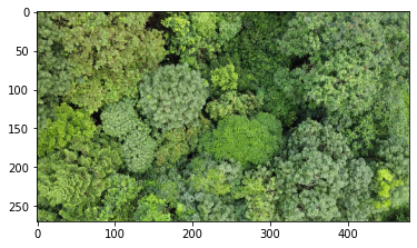
Read the image and divide it by 16 to reduce runtime

ar = imread("../../../data/image.jpg")[::4, ::4]
plt.imshow(ar)

<matplotlib.image.AxesImage at 0x22649abaaf0>

GLCM Transformation

Option 1: Use GLCM to transform

We load GLCM, Direction and Features. The latter 2, self-explanatory, to specify arguments

• Set directions to only East & South East

• Set features to run only ASM & Contrast.

• Bin from 256 to 16, reducing run time

• Normalize Features to [0, 1]

• Allow tqdm to output progress

• Set Step Size to 1, Radius to 2.

from glcm_cupy import GLCM, Direction, Features

g = GLCM(
    directions=(Direction.EAST, Direction.SOUTH_EAST),
    features=(Features.ASM, Features.CONTRAST),
    bin_from=256, bin_to=16,
    normalized_features=True,
    verbose=True,
    step_size=1,
    radius=2
).run(ar)

GLCM Progress: 100%|██████████| 751k/751k [00:01<00:00, 656k Cells/s] 

Option 2: Use glcm to transform

Alternatively, use the functional call

Notice how the number of cells is doubled, because by default, we use 4 directions!

from glcm_cupy import glcm

ar_g = glcm(ar, bin_from=256, bin_to=16)  # Argument names are the same

GLCM Progress: 100%|██████████| 1.50M/1.50M [00:04<00:00, 350k Cells/s]

Feature Extraction

After Transformation, extract features

Option 1: Extract Features with Features

Each 2D channel is transformed into its own 2D GLCM Feature channel, with reduced height & width

# We yield the features using constants defined in conf
from glcm_cupy.conf import Features

print(ar_g[..., Features.CONTRAST].shape, ar_g[..., Features.CORRELATION].shape, ar_g[..., Features.ASM].shape)

(264, 474, 3) (264, 474, 3) (264, 474, 3)

Option 2: Extract Features with integers

Alternatively, since these constants are simply integers

You may inspect the source of Features to yield the integers

print(ar_g[..., 0].shape, ar_g[..., 1].shape, ar_g[..., 2].shape)

(264, 474, 3) (264, 474, 3) (264, 474, 3)

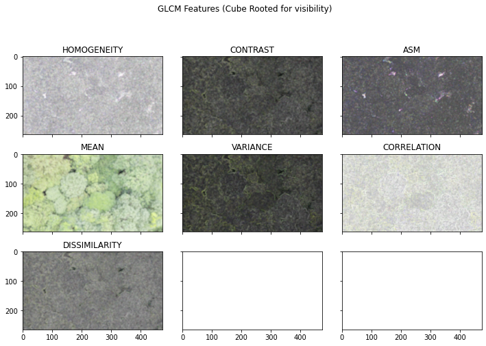
Plot Transformation

Plot features with ImageGrid.

Some features have extremely low values, thus we cube root it to spread it out.

# Plot in a grid
fig = plt.figure(figsize=(12, 8))
grid = ImageGrid(fig, 111,
                 nrows_ncols=(3, 3),
                 axes_pad=0.4)

for ax, f_ix, title in zip(grid, range(ar_g.shape[-1]),
                           ("HOMOGENEITY", "CONTRAST", "ASM", "MEAN",
                            "VARIANCE", "CORRELATION", "DISSIMILARITY"), ):
    ax.imshow(ar_g[..., f_ix] ** (1 / 3))
    ax.set_title(title)
fig.suptitle('GLCM Features (Cube Rooted for visibility)')

Text(0.5, 0.98, 'GLCM Features (Cube Rooted for visibility)')

Summary

• You have learnt how GLCM and glcm transforms the image array

• The input criterion

• How to extract features

• The shape shrink of GLCM

Things to Note

Not all features are significantly orthogonal.

It’s best to research on which features to use or do feature selection to reduce run time of GLCM.